This notebook benchmarks NDIndex performance for various operations and dataset sizes. Understanding performance characteristics helps you make informed decisions about when and how to use NDIndex in your workflows.
import time

import matplotlib.pyplot as plt
import numpy as np
import pandas as pd
import xarray as xr

from linked_indices import NDIndex
Benchmark Utilities
def benchmark(func, n_runs=100, warmup=5):
    """Benchmark a function and return timing statistics."""
    # Warmup runs
    for _ in range(warmup):
        func()

    # Timed runs
    times = []
    for _ in range(n_runs):
        start = time.perf_counter()
        func()
        end = time.perf_counter()
        times.append(end - start)

    times = np.array(times)
    return {
        "mean": times.mean(),
        "std": times.std(),
        "min": times.min(),
        "max": times.max(),
        "median": np.median(times),
    }


def create_dataset(n_trials, n_times):
    """Create a test dataset with given dimensions."""
    trial_onsets = np.arange(n_trials) * n_times * 0.01
    rel_time = np.linspace(0, n_times * 0.01, n_times)

    abs_time = trial_onsets[:, np.newaxis] + rel_time[np.newaxis, :]
    data = np.random.randn(n_trials, n_times)

    ds = xr.Dataset(
        {"data": (["trial", "rel_time"], data)},
        coords={
            "trial": np.arange(n_trials),
            "rel_time": rel_time,
            "abs_time": (["trial", "rel_time"], abs_time),
        },
    )
    return ds.set_xindex(["abs_time"], NDIndex)
1. Index Creation Performance
How long does it take to create an NDIndex for datasets of different sizes?
# Test different dataset sizes
sizes = [
    (10, 100),  # 1K cells
    (10, 1000),  # 10K cells
    (100, 1000),  # 100K cells
    (100, 10000),  # 1M cells
    (1000, 10000),  # 10M cells
]

creation_results = []
for n_trials, n_times in sizes:
    n_cells = n_trials * n_times

    # Create base dataset without index
    trial_onsets = np.arange(n_trials) * n_times * 0.01
    rel_time = np.linspace(0, n_times * 0.01, n_times)
    abs_time = trial_onsets[:, np.newaxis] + rel_time[np.newaxis, :]
    data = np.random.randn(n_trials, n_times)

    ds_base = xr.Dataset(
        {"data": (["trial", "rel_time"], data)},
        coords={
            "trial": np.arange(n_trials),
            "rel_time": rel_time,
            "abs_time": (["trial", "rel_time"], abs_time),
        },
    )

    # Benchmark index creation
    result = benchmark(lambda: ds_base.set_xindex(["abs_time"], NDIndex), n_runs=50)
    result["n_cells"] = n_cells
    result["n_trials"] = n_trials
    result["n_times"] = n_times
    creation_results.append(result)

    print(
        f"{n_trials:4d} trials × {n_times:5d} times ({n_cells:>8,} cells): {result['mean'] * 1000:>8.3f} ms"
    )
10 trials × 100 times ( 1,000 cells): 0.006 ms
10 trials × 1000 times ( 10,000 cells): 0.006 ms
100 trials × 1000 times ( 100,000 cells): 0.006 ms
100 trials × 10000 times (1,000,000 cells): 0.006 ms
1000 trials × 10000 times (10,000,000 cells): 0.006 ms
# Plot creation times
df = pd.DataFrame(creation_results)

fig, ax = plt.subplots(figsize=(8, 5))

# Use bar chart to show creation is essentially constant
x_labels = [f"{r['n_cells']:,}" for r in creation_results]
ax.bar(x_labels, df["mean"] * 1000)
ax.set_xlabel("Number of cells")
ax.set_ylabel("Index creation time (ms)")
ax.set_title("NDIndex Creation Performance")
ax.set_ylim(0, max(df["mean"] * 1000) * 1.5)  # Start at 0 to show how small these are

# Add text showing the actual values
for i, (x, y) in enumerate(zip(x_labels, df["mean"] * 1000)):
    ax.text(i, y + 0.0005, f"{y:.3f}", ha="center", fontsize=9)

plt.tight_layout()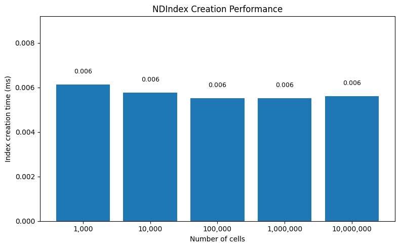
Key insight: NDIndex creation is O(1) - it just stores a reference to the coordinate array. No preprocessing or tree-building is required.
2. Scalar Selection Performance
How long does sel(abs_time=value, method='nearest') take?
scalar_results = []

for n_trials, n_times in sizes:
    n_cells = n_trials * n_times
    ds = create_dataset(n_trials, n_times)

    # Pick a random target value in the middle of the range
    target = float(ds.abs_time.values.mean())

    # Benchmark scalar selection
    result = benchmark(lambda: ds.sel(abs_time=target, method="nearest"), n_runs=100)
    result["n_cells"] = n_cells
    scalar_results.append(result)

    print(
        f"{n_cells:>10,} cells: {result['mean'] * 1000:>8.3f} ms (±{result['std'] * 1000:.3f})"
    )
1,000 cells: 0.056 ms (±0.017)
10,000 cells: 0.071 ms (±0.018)
100,000 cells: 0.259 ms (±0.173)
1,000,000 cells: 3.969 ms (±7.272)
10,000,000 cells: 25.385 ms (±3.130)
# Plot scalar selection times
df_scalar = pd.DataFrame(scalar_results)

fig, ax = plt.subplots(figsize=(8, 5))
ax.loglog(
    df_scalar["n_cells"], df_scalar["mean"] * 1000, "o-", markersize=8, label="Measured"
)

# Add O(n) reference line (anchored to largest size to show theoretical worst case)
x_ref = np.array([df_scalar["n_cells"].min(), df_scalar["n_cells"].max()])
y_ref = df_scalar["mean"].iloc[-1] * 1000 * (x_ref / x_ref[-1])
ax.plot(x_ref, y_ref, "--", color="gray", alpha=0.5, label="O(n) reference")

ax.set_xlabel("Number of cells")
ax.set_ylabel("Selection time (ms)")
ax.set_title("Scalar Selection Performance (method='nearest')")
ax.grid(True, alpha=0.3)
ax.legend()

plt.tight_layout()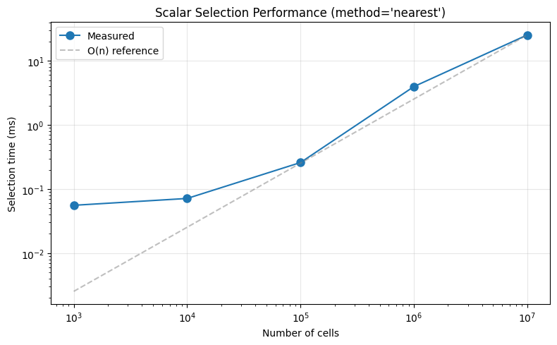
Key insights:
Fixed overhead dominates at small sizes (~0.06ms for xarray machinery, index lookup, result construction)
Scaling is O(n) for large arrays - from 100K to 10M cells (100× increase), time increases ~100× as expected
NumPy makes O(n) fast -
np.argminuses SIMD vectorization and cache-efficient memory access, so even 10M cells only takes ~25ms
Bottom line: The algorithm is O(n), but numpy’s optimizations make the constant factor very small. For typical neuroscience datasets (<1M cells), selection is effectively instant (~1-2ms).
3. Slice Selection Performance
How long does sel(abs_time=slice(start, stop)) take?
slice_results = []

for n_trials, n_times in sizes:
    n_cells = n_trials * n_times
    ds = create_dataset(n_trials, n_times)

    # Select middle 50% of the data
    vmin, vmax = ds.abs_time.values.min(), ds.abs_time.values.max()
    start = vmin + (vmax - vmin) * 0.25
    stop = vmin + (vmax - vmin) * 0.75

    # Benchmark slice selection
    result = benchmark(lambda: ds.sel(abs_time=slice(start, stop)), n_runs=100)
    result["n_cells"] = n_cells
    slice_results.append(result)

    print(
        f"{n_cells:>10,} cells: {result['mean'] * 1000:>8.3f} ms (±{result['std'] * 1000:.3f})"
    )
1,000 cells: 0.084 ms (±0.142)
10,000 cells: 0.062 ms (±0.004)
100,000 cells: 0.135 ms (±0.008)
1,000,000 cells: 0.904 ms (±0.080)
10,000,000 cells: 9.108 ms (±1.296)
# Compare scalar vs slice selection
df_slice = pd.DataFrame(slice_results)

fig, ax = plt.subplots(figsize=(8, 5))
ax.loglog(
    df_scalar["n_cells"],
    df_scalar["mean"] * 1000,
    "o-",
    markersize=8,
    label="Scalar selection",
)
ax.loglog(
    df_slice["n_cells"],
    df_slice["mean"] * 1000,
    "s-",
    markersize=8,
    label="Slice selection",
)

ax.set_xlabel("Number of cells")
ax.set_ylabel("Selection time (ms)")
ax.set_title("Selection Performance Comparison")
ax.grid(True, alpha=0.3)
ax.legend()

plt.tight_layout()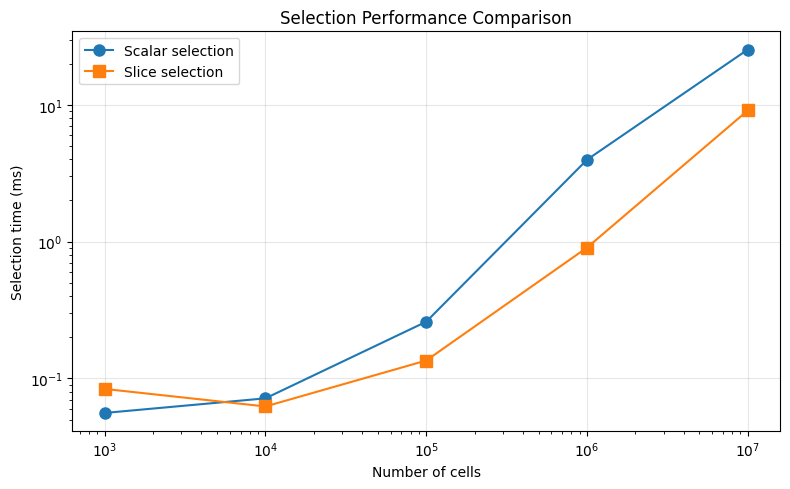
4. isel Performance
How does NDIndex affect isel() performance? This matters because
isel() needs to slice the internal coordinate arrays.
isel_results = []

for n_trials, n_times in sizes:
    n_cells = n_trials * n_times
    ds = create_dataset(n_trials, n_times)

    # Also create version without NDIndex for comparison
    ds_no_index = ds.drop_indexes("abs_time")

    # Benchmark isel with NDIndex
    result_with = benchmark(lambda: ds.isel(trial=0), n_runs=100)
    result_without = benchmark(lambda: ds_no_index.isel(trial=0), n_runs=100)

    isel_results.append(
        {
            "n_cells": n_cells,
            "with_index": result_with["mean"],
            "without_index": result_without["mean"],
            "overhead": result_with["mean"] / result_without["mean"],
        }
    )

    print(
        f"{n_cells:>10,} cells: with={result_with['mean'] * 1000:.3f}ms, without={result_without['mean'] * 1000:.3f}ms, overhead={result_with['mean'] / result_without['mean']:.2f}x"
    )
1,000 cells: with=0.036ms, without=0.027ms, overhead=1.34x
10,000 cells: with=0.031ms, without=0.024ms, overhead=1.29x
100,000 cells: with=0.036ms, without=0.029ms, overhead=1.22x
1,000,000 cells: with=0.031ms, without=0.025ms, overhead=1.27x
10,000,000 cells: with=0.036ms, without=0.024ms, overhead=1.48x
df_isel = pd.DataFrame(isel_results)

fig, axes = plt.subplots(1, 2, figsize=(12, 5))

ax = axes[0]
ax.loglog(df_isel["n_cells"], df_isel["with_index"] * 1000, "o-", label="With NDIndex")
ax.loglog(
    df_isel["n_cells"], df_isel["without_index"] * 1000, "s-", label="Without NDIndex"
)
ax.set_xlabel("Number of cells")
ax.set_ylabel("isel() time (ms)")
ax.set_title("isel() Performance")
ax.legend()
ax.grid(True, alpha=0.3)

ax = axes[1]
ax.semilogx(df_isel["n_cells"], df_isel["overhead"], "o-")
ax.axhline(1, color="gray", linestyle="--", alpha=0.5)
ax.set_xlabel("Number of cells")
ax.set_ylabel("Overhead factor")
ax.set_title("NDIndex isel() Overhead")
ax.grid(True, alpha=0.3)

plt.tight_layout()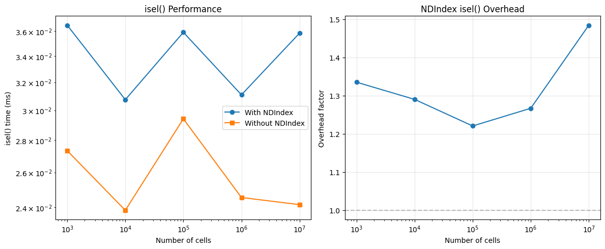
5. Memory Usage
NDIndex stores references to coordinate arrays, not copies. Let’s verify the memory overhead is minimal.
# Create a large dataset
n_trials, n_times = 100, 10000
n_cells = n_trials * n_times

trial_onsets = np.arange(n_trials) * n_times * 0.01
rel_time = np.linspace(0, n_times * 0.01, n_times)
abs_time = trial_onsets[:, np.newaxis] + rel_time[np.newaxis, :]
data = np.random.randn(n_trials, n_times)

ds_base = xr.Dataset(
    {"data": (["trial", "rel_time"], data)},
    coords={
        "trial": np.arange(n_trials),
        "rel_time": rel_time,
        "abs_time": (["trial", "rel_time"], abs_time),
    },
)

ds_indexed = ds_base.set_xindex(["abs_time"], NDIndex)

# Check if the arrays share memory
print(f"Dataset size: {n_cells:,} cells")
print(f"abs_time array size: {abs_time.nbytes / 1024 / 1024:.2f} MB")
print(
    f"Arrays share memory: {np.shares_memory(ds_base.abs_time.values, ds_indexed.abs_time.values)}"
)
Dataset size: 1,000,000 cells
abs_time array size: 7.63 MB
Arrays share memory: True
6. Comparison: Multiple Coordinates
How does performance scale when indexing multiple N-D coordinates?
# Create dataset with multiple 2D coordinates
n_trials, n_times = 100, 1000
n_cells = n_trials * n_times

trial_onsets = np.arange(n_trials) * 10.0
rel_time = np.linspace(0, 5.0, n_times)
abs_time = trial_onsets[:, np.newaxis] + rel_time[np.newaxis, :]

# Create event-locked coordinates
event1_times = np.random.uniform(1, 2, n_trials)
event2_times = np.random.uniform(2, 3, n_trials)
event1_locked = rel_time[np.newaxis, :] - event1_times[:, np.newaxis]
event2_locked = rel_time[np.newaxis, :] - event2_times[:, np.newaxis]

ds_multi = xr.Dataset(
    {"data": (["trial", "rel_time"], np.random.randn(n_trials, n_times))},
    coords={
        "trial": np.arange(n_trials),
        "rel_time": rel_time,
        "abs_time": (["trial", "rel_time"], abs_time),
        "event1_locked": (["trial", "rel_time"], event1_locked),
        "event2_locked": (["trial", "rel_time"], event2_locked),
    },
)

print("Benchmarking with 1, 2, and 3 indexed coordinates...")
print()

# Index different numbers of coordinates
for n_coords, coords in [
    (1, ["abs_time"]),
    (2, ["abs_time", "event1_locked"]),
    (3, ["abs_time", "event1_locked", "event2_locked"]),
]:
    ds_test = ds_multi.set_xindex(coords, NDIndex)

    # Benchmark selection on first coordinate
    target = float(ds_test.abs_time.values.mean())
    result = benchmark(
        lambda: ds_test.sel(abs_time=target, method="nearest"), n_runs=100
    )

    print(f"{n_coords} coord(s): sel() = {result['mean'] * 1000:.3f} ms")
Benchmarking with 1, 2, and 3 indexed coordinates...
1 coord(s): sel() = 0.189 ms
2 coord(s): sel() = 0.170 ms
3 coord(s): sel() = 0.167 ms
Summary
Performance Characteristics
| Operation | Complexity | Notes |
|---|---|---|
| Index creation | O(1) | Just stores reference, no preprocessing |
| Scalar selection (nearest) | O(n) | Linear scan with np.argmin |
| Scalar selection (exact) | O(n) | Linear scan with np.where |
| Slice selection | O(n) | Boolean masking + bounding box computation |
isel() | O(1) | Array slicing is fast |
Recommendations
Small-medium datasets (<1M cells): NDIndex adds negligible overhead
Large datasets (1-10M cells): Selection takes ~10-100ms, usually acceptable
Very large datasets (>10M cells): Consider:
Pre-filtering with
isel()beforesel()Using exact matching instead of nearest-neighbor
Chunking your data with dask
Memory: NDIndex doesn’t copy data, so memory overhead is minimal